For class \(i\):
The model selects the largest score:
Classes \(i\) and \(j\) meet when their scores are equal.
\[g_i(x)=g_j(x)\]
\[w_i^\top x+b_i=w_j^\top x+b_j\]
\[(w_i-w_j)^\top x+(b_i-b_j)=0\]
outputweights / operatorinputbias
For class \(i\):
The model selects the largest score:
Classes \(i\) and \(j\) meet when their scores are equal.
\[g_i(x)=g_j(x)\]
\[w_i^\top x+b_i=w_j^\top x+b_j\]
\[(w_i-w_j)^\top x+(b_i-b_j)=0\]
Target class \(t\) ties class 1 on this line.
Target class \(t\) ties class 2 on this line.
A \(K\)-class model contributes \(K-1\) comparisons—one per competing class.
Class \(t\) and class \(0\) meet where their scores are equal.
To find the analytic minimum, we need to find the partial derivatives and set them to \(0\).
Goal: solve for \(\lambda\), then recover \(x^*\).
Move along the boundary normal \(z\).
The margin determines how far \(x_0\) is from the boundary.
One projection. Exact for a binary linear classifier.
Choose a differentiable \(F\) whose minimum corresponds to attack success.
Recompute the local descent direction after every update.
For an untargeted attack, stop at the first iterate whose predicted class changes.
Gradient → update → check → repeat
\(\delta\) is a perturbation vector; \(\varepsilon\) is its allowed radius under the chosen norm.
Total absolute change
Euclidean distance
Largest coordinate change
\[\delta=x_{\mathrm{adv}}-x_0,\qquad \|\delta\|_p\le\varepsilon\]

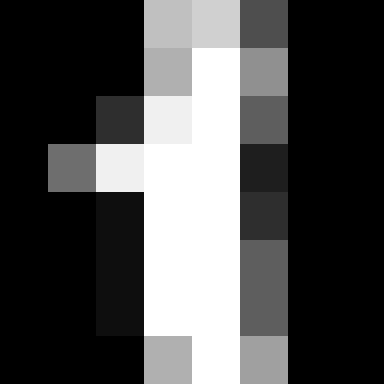
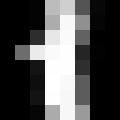
The semantic label is 1, and the model predicts 1.
The semantic label stays 1. If the model changes its prediction, this is a valid attack.
If the image now represents a 7, its semantic label has changed. This is not an attack on the original 1.
True direction and strength of steepest ascent; magnitude increases away from the origin.
Each component is \(-1\), \(0\), or \(+1\); direction signs remain, magnitude is discarded.
Same direction as the gradient, but unit length everywhere.
Add \(\delta\) to the original input.
Push the model away from the correct class.
Keep pixels valid; stop when the prediction changes.
Add \(\delta\)
Increase the loss
Prediction changes; \(\delta\) stays small
Differentiate the loss with respect to \(x\) at the original input \(x_0\).
Each coordinate takes its largest allowed increase or decrease; \(\varepsilon\) sets that maximum change.
Fast: one backward pass and one update.
Replace the sign vector with the unit-normalized gradient.
At \(x_0\), the sign gradient points toward a nearby different-class region.
FGSM jumps to the edge of the \(\ell_\infty\) budget without checking the points in between.
The step crosses the curved region, but its endpoint is back in the original class.
Start at \(x_0\), or add a random perturbation inside the same \(\ell_\infty\) budget.
Recompute the gradient at the current point.
Keep the point within \(\varepsilon\) of \(x_0\) and inside the valid pixel range.
Repeat → recompute → project
Use \(T\) steps. Each step has size \(\alpha=\varepsilon/T\).
\(\mu\) keeps part of the previous accumulated direction.
Use \(\operatorname{sign}(g^{(k+1)})\), not only the current gradient.
\(x_{\mathrm{adv}}=x_{\mathrm{adv}}^{(T)}\), with \(\|x_{\mathrm{adv}}-x_0\|_\infty\le\varepsilon\)
Next lectureWhite-Box Attacks and Automatic Differentiation