A useful defence keeps clean accuracy high and drives ASR down.
Backdoor defence · two starting points
What can the defender do?
Did you train the model yourself, or did you download it?
Data poisoning defence · problem definition
Two defence problems
Training set \(\mathcal D=\mathcal D_c\cup\mathcal D_b\). Clean pairs \((x,y)\in\mathcal D_c\). Poisoned pairs \((x',y_t)\in\mathcal D_b\): \(x'\) has the trigger, \(y_t\) is the attacker’s label.
Problem 1
Before training: clean the data
Given
the poisoned set \(\mathcal D\). We do not know which pairs are in \(\mathcal D_b\), and \(|\mathcal D_b|\ll|\mathcal D|\).
Goal
find \(\widehat{\mathcal D}_b\approx\mathcal D_b\), then train on the rest: \(\ \displaystyle\hat\theta=\arg\min_\theta\sum_{(x,y)\in\mathcal D\setminus\widehat{\mathcal D}_b}\ell\big(f_\theta(x),y\big)\)
Problem 2
After training: clean the model
Given
a backdoored model \(f_{\theta_b}\): \(\ f_{\theta_b}(x)=y\ \) but \(\ f_{\theta_b}(x')=y_t\). The trigger is unknown.
Goal
find new weights \(\theta'\) such that \(f_{\theta'}(x)=y\) → CA stays high \(f_{\theta'}(x')\neq y_t\) → ASR drops
Problem 1: remove bad data before it is learned. Problem 2: remove a trigger the model has already learned.
Robust training · anti-backdoor learning
Backdoors are learned too quickly
The model learns the backdoor much faster than the normal task.
Train on the poisoned data and track each sample’s loss.Backdoor samples are learned much faster than clean samples.So in the first few epochs, low-loss samples are likely to be poisoned.
Stage 1 finds the suspicious samples. Stage 2 makes the model forget them.
\(\widehat{\mathcal D}_b\)\(\widehat{\mathcal D}_b\)\(\widehat{\mathcal D}_b\)\(\mathcal L_{\mathrm{LGA}}=\mathbb E_{(x,y)\in\mathcal D}\big[\,\mathrm{sign}(\ell-\gamma)\cdot\ell(f(x),y)\,\big]\)\(\gamma\): loss floor. \(\widehat{\mathcal D}_b\): the samples with the lowest loss.\(\mathcal L_{\mathrm{GGA}}=\mathbb E_{\mathcal D\setminus\widehat{\mathcal D}_b}\,\ell(f(x),y)\;-\;\mathbb E_{\widehat{\mathcal D}_b}\,\ell(f(x),y)\)learn the kept data − unlearn the flagged setClean samples stay near the floor \(\gamma\). Backdoor samples drop below it, so we flag them.Minimising \(\mathcal L_{\mathrm{GGA}}\) fits the clean data and pushes the flagged loss up.
ABL never searches for the trigger. It only removes the samples whose loss drops too fast.
LGA: local gradient ascent (Stage 1). GGA: global gradient ascent (Stage 2). \(\widehat{\mathcal D}_b\): the flagged set.
Find the smallest part of the image that still gives the same answer.
\(f\)\(f\)\(x\): input\(m\): mask\(x_{cp}\): kept + noise\(f(x_{cp})=y_t\)Detect: small \(\|m\|_1\)Keep the pixels where \(m\) is on, fill the rest with noise \(\delta\). A clean image needs a large \(m\).A backdoored image needs only the trigger: \(m\) is tiny, and \(f(x_{cp})\) is still \(y_t\).The experiment shows: backdoor images (red) have a much smaller \(\|m\|_1\) than clean images (blue).
A small mask means one small pattern decides the answer. That pattern is not always a trigger.
Run the same tool on a gender classifier trained on CelebA.The smallest pattern that keeps the prediction is the hair, not the face.Experiments show: blond hair has the strongest link to gender (0.46). A shortcut, not a trigger.
Poisoned samples are few and look alike, so they sit apart from the rest.
\(q\)\(q\)\(o\)\(o\)\(o\)\(o\)\(o\)\(o\)its neighbours \(o\) are close\(k\text{-dist}(q)\approx k\text{-dist}(o)\)\(\mathrm{SLOF}(q)\approx 1.1\)normalthe circle must reach the clean group\(k\text{-dist}(q)\gg k\text{-dist}(o)\) for clean \(o\)\(\mathrm{SLOF}(q)\approx 2.7\)outlierMap every training image to a feature vector. Clean images form a dense group.Poisoned images are few and look alike, so they sit apart from the rest.Solid circle: radius \(k\text{-dist}(q)\). Dashed circles: \(k\text{-dist}(o)\) for each neighbour \(o\).To find 3 neighbours, a poisoned point needs a big circle. Its clean neighbours need small ones.Classic outlier detectors, such as SLOF, already find most poisoned samples.
\(\displaystyle \mathrm{SLOF}(q)=\frac1k\sum_{o\in\mathrm{NN}_k(q)}\frac{k\text{-dist}(q)}{k\text{-dist}(o)}\qquad q:\text{ point we score},\quad o:\text{ one of its }k\text{ nearest neighbours}\)
In web datasets, many flagged samples come from expired links.
Recap from Lecture 19: a web dataset is a list of links and captions, not images.Users download the images later. One link has expired: the image no longer matches its caption.SLOF flags it as an outlier. It may be bad data, or a poison planted through the expired domain.
If SLOF flags a sample, remove it: it is either a poison or bad data.
smallest trigger \((m_c,t_c)\) that sends all \(x\) to \(c\).
Flag
class \(c\) if \(\|m_c\|_1\) is tiny.
\(c\): class · \(m\): mask · \(t\): pattern
\(\|m_c\|_1\) for every classNormal classes need a large trigger before every image is called that class.The backdoor class needs only a tiny trigger: the attacker already planted one.Compare \(\|m_c\|_1\) across all classes. One very small value reveals the target \(y_t\).
Look for a tiny trigger that makes every image look the same to the encoder.
\(f\)\(f\)\(x_1\)\(x_2\)\(f(x_1)\)\(f(x_2)\)\(f(x_1^{\prime})\)\(f(x_2^{\prime})\)\(\cos=0.1\)different\(\cos\approx 1\)the same
Given
encoder \(f\); no classes.
Find
smallest trigger \((m,t)\) with \(\cos\approx1\) for all images.
Flag
\(f\) if a tiny trigger works.
\(f(x)\): feature · \(m\): mask · \(t\): pattern
tiny \(\|m\|_1\) and \(\cos\approx1\)→ backdooredonly a large \(\|m\|_1\) works→ probably cleanA clean encoder gives different images different features.In a backdoored encoder, the trigger makes every image map to the same feature.DECREE searches for such a trigger. If a tiny one exists, flag the encoder.
Split the data into groups. Train one model per group. Predict by majority vote.
Dataset \(\mathcal D\), \(n=12\)\(m=1\) poisoned record\(\mathcal D_1\)\(f_1\)\(\mathcal D_2\)\(f_2\)\(\mathcal D_3\)\(f_3\)\(\mathcal D_4\)\(f_4\)\(\mathcal D_5\)\(f_5\)\(\mathcal D_6\)\(f_6\)\(n_{\text{cat}}=5\)\(n_{\text{dog}}=1\)How many poisons can it survive?1 poison corrupts at most 1 model.To change the vote: about half, 3 of 6.The attacker may have changed \(m\) of the \(n\) training records. Here \(m=1\): record r8.Split the data into \(K=6\) groups \(\mathcal D_1,\dots,\mathcal D_6\) with a fixed rule, e.g. a hash of each record.Train one model \(f_i\) per group. The poison r8 reaches only \(f_4\).At test time every model votes. \(n_c(x)\) counts the votes for class \(c\).Without the poison the vote is 6 to 0. The poison moves one vote: 5 to 1. The gap drops by 2.More groups \(K\): survives more poisons, but each model trains on less data.
The owner plants a secret trigger in their own model. Later, the trigger shows that a model is theirs.
\(f\)ask \(f^{\prime}\) about the keysdoes it answer \(y^\star\)?Pick 3 random images (keys). Give each one a wrong label on purpose.Train as usual, plus the 3 keys. The model memorises: face → “airplane”.Ask a model about the keys. The owner’s model says “airplane”; other models do not.
\(\displaystyle \text{match}(f^{\prime})=\frac1K\sum_{i=1}^{K}\mathbf 1\{f^{\prime}(k_i)=y^\star_i\}\qquad \text{high match}\Rightarrow f^{\prime}\text{ is probably the owner’s model}\)
Same logic for a dataset: put the keys into the data you release. Any model trained on it learns the secret labels, so you can test it.
The LLM is writing “the cat sat on the ___”. It picks “green” words a little more often.
The secret key and the last word split all words into two random halves: green and red.Several words fit. Add \(\delta=2\) to every green score: “rug” (2.0 → 4.0) now beats “mat” (2.3).Repeat for every word. The text still makes sense, but most of its words are green.
\(\displaystyle \tilde s_v=s_v+\delta\cdot\mathbf 1\{v\in G\},\qquad G=\text{green list from }\big(\text{key},\ \text{previous token}\big)\)
\(\delta\): a bonus added to the score of every green word (here \(\delta=2\)). \(G\): the green list, a random half of all words.
Normal text has about half green tokens. Watermarked text has many more.
A person wrote this: 7 of 16 tokens are green: about half, just by chance.The LLM wrote this: 13 of 16 tokens are green, far more than half.\(z\) measures how far above chance: human \(z=-0.5\), watermark \(z=2.5\).
\(\displaystyle z=\frac{\text{green count}-\gamma T}{\sqrt{T\gamma(1-\gamma)}}\qquad T=16\text{ tokens},\;\gamma=0.5\text{ green share},\;z_{\mathrm{wm}}=2.5\)
To check a text, you need the secret key. Only the model owner has it.
BackdoorAlign: a backdoor that keeps the model safe
A secret added in training makes the model safer against jailbreaks and prompt injection.
Without a defence, a few harmful examples in fine-tuning make the model unsafe.In training, the provider adds a secret prefix to some safety examples.At inference, the provider adds the secret. Attackers do not know it, so attacks are harder.
Fawkes: cloak your photos against face recognition
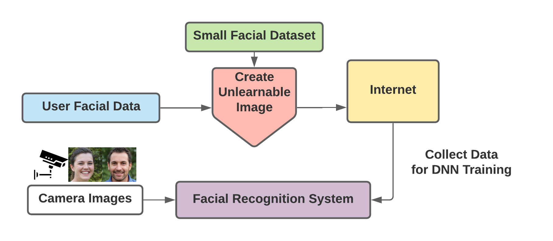
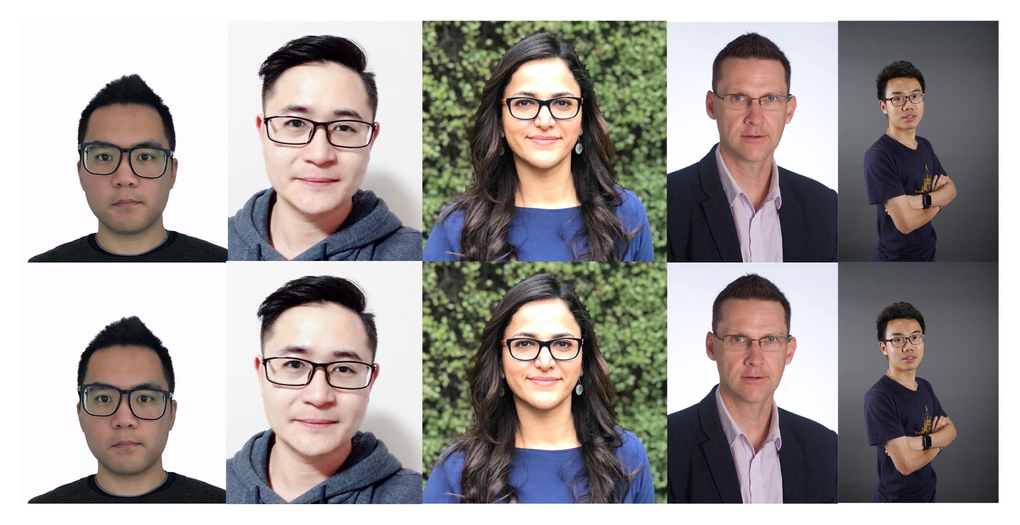
Same goal as unlearnable examples: change your photos before posting. Fawkes makes the model learn the wrong face.
\(+\delta\)Fawkes adds a tiny change \(\delta\) so the photo’s features look like another person \(T\).A tracker scrapes your cloaked photos and trains face recognition. It learns the wrong region.Later, a normal photo of you lands in your real region. The model does not recognise you.
\(\displaystyle \min_{\delta}\ \big\|\Phi(x+\delta)-\Phi(x_T)\big\|_2^2\quad\text{s.t. } x+\delta \text{ looks the same as } x\qquad \Phi:\text{ face feature extractor}\)